Lesson 6: Compute new data attributes
Preparation
If not the case yet, load the demo dataset and start the 'Trends and Distributions' Cockpit, as described in the beginning of lesson 01.
At any time, additional data attributes can be added to the analysis. A formula editor supports everything from typing simple arithmetic formulas, to complex Python 3 scripts. Optionally, there are several built-in formula blocks ready to use.
Creating your first new numerical time series
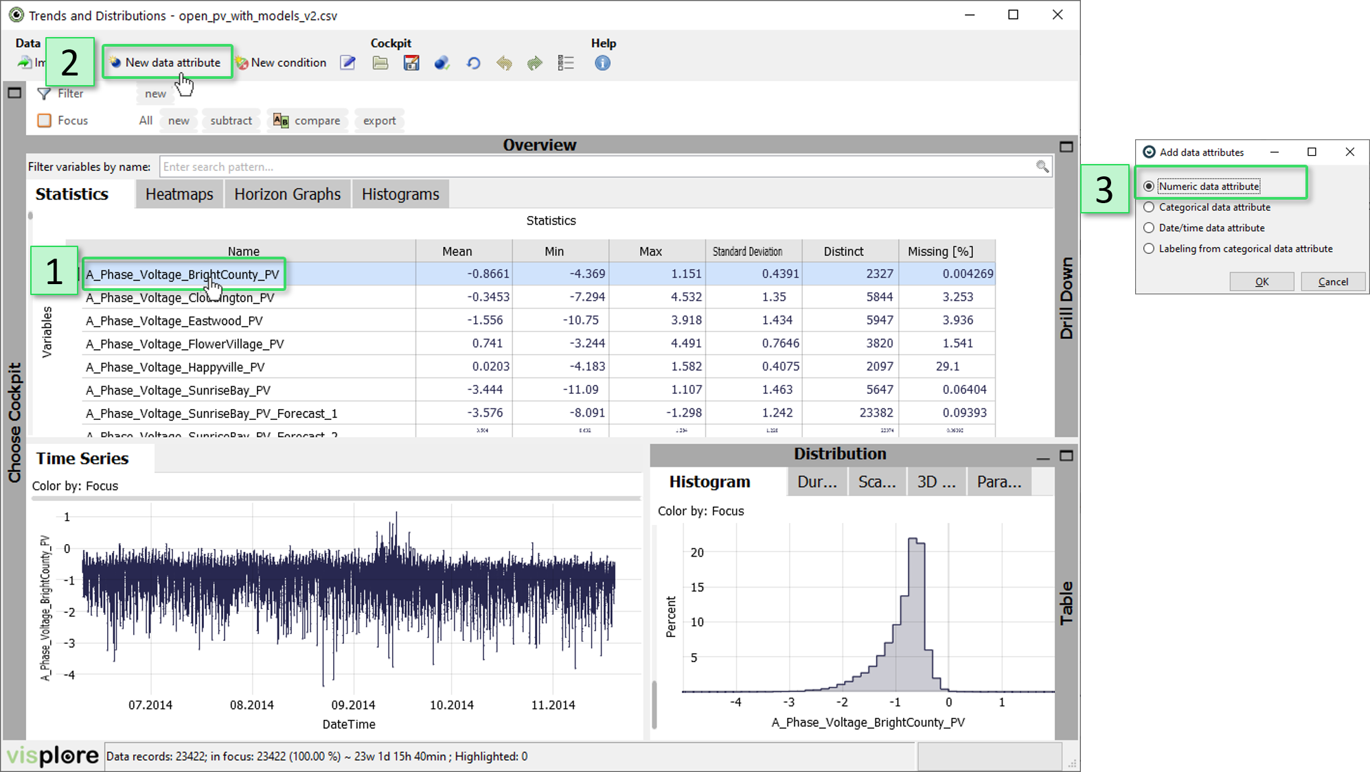
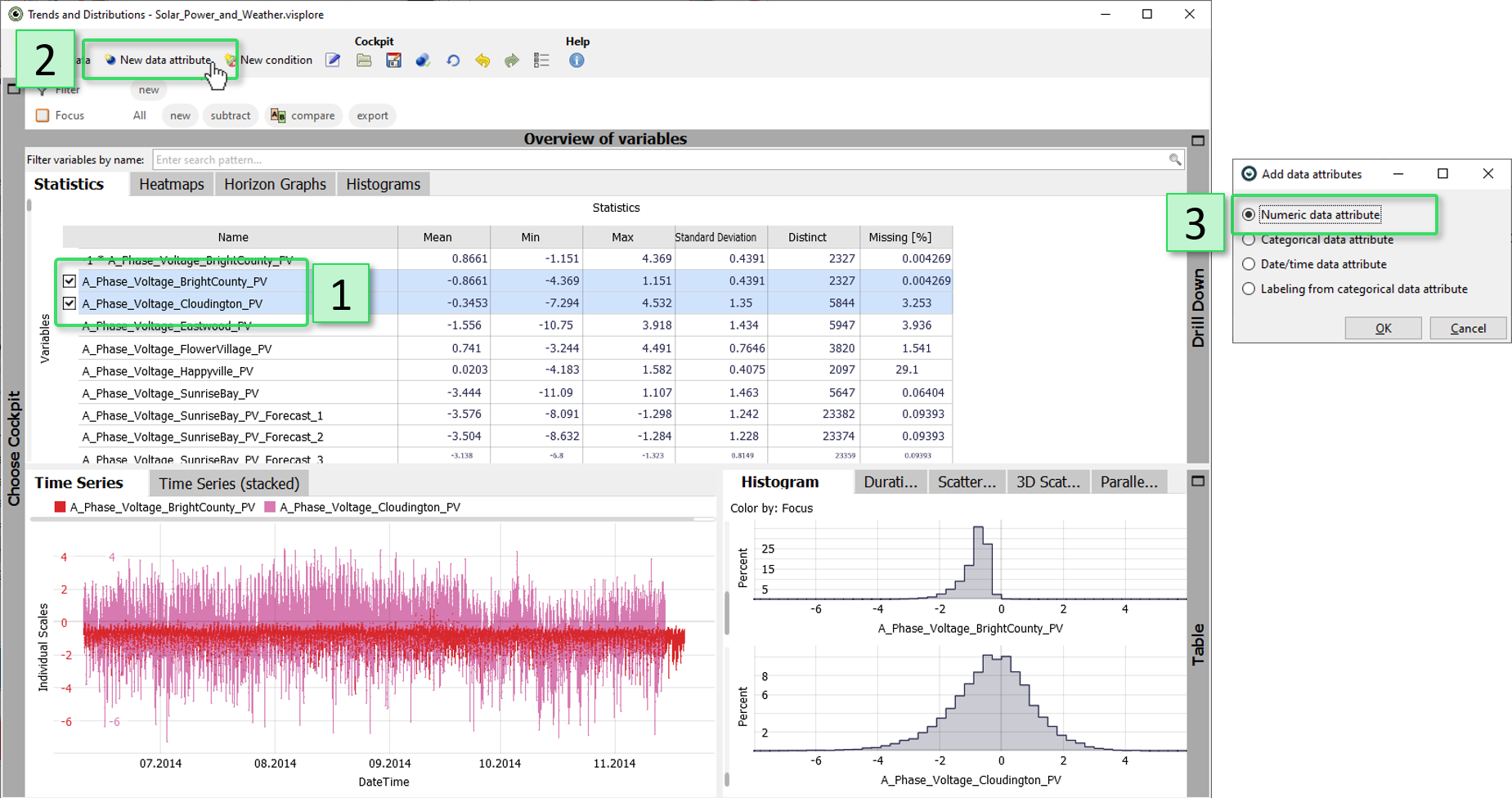
1. Select the first time series "A_Phase_Voltage_BrightCounty_PV" in the "Statistics" view by clicking its name. This will be the input to the newly computed time series.
2. Then, click "New data attribute" in the toolbar.
3. Select "Define numeric data attribute" from the dialog. Alternatively, a categorical attribute can be created using the same workflow, which you can try out later. Press "OK".
|
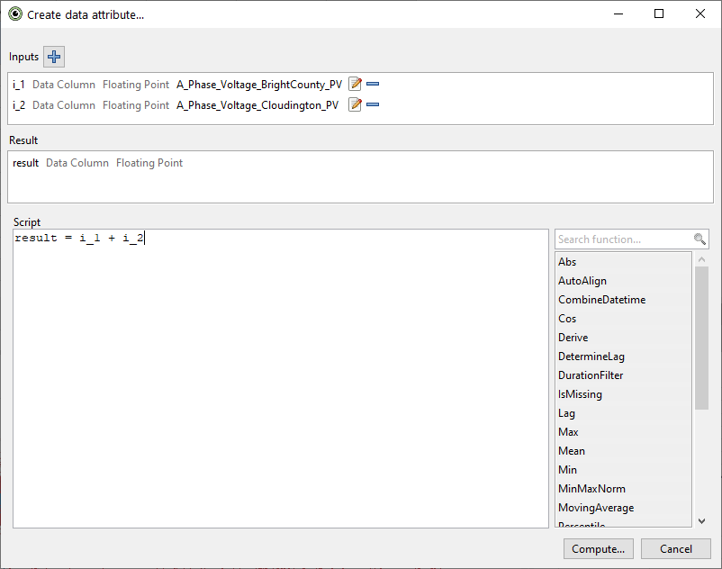
The next dialog is the formula editor. These are the most important elements:
|
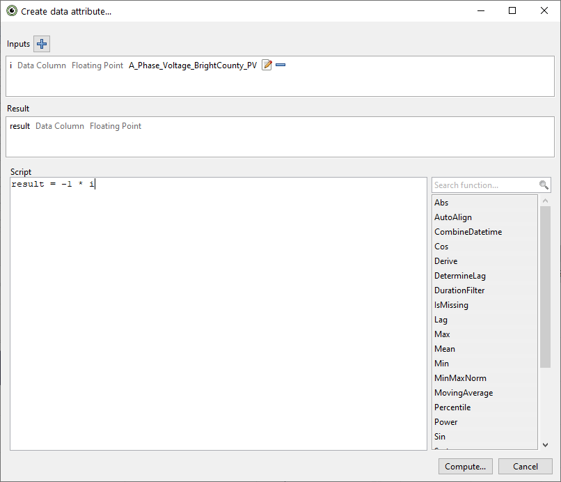 |
Our first computation will be inverting the sign of the values. In other words, multiplying the values by -1. Click in the "Script" field, and type: result = -1 * i
Click "Compute".
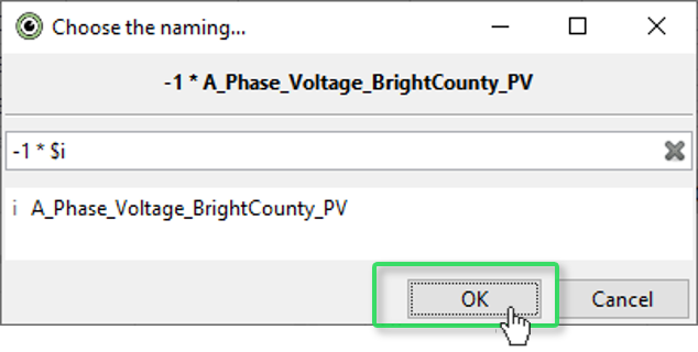
The next dialog is for naming the new attribute. For now, accept the suggested name, and press "OK".
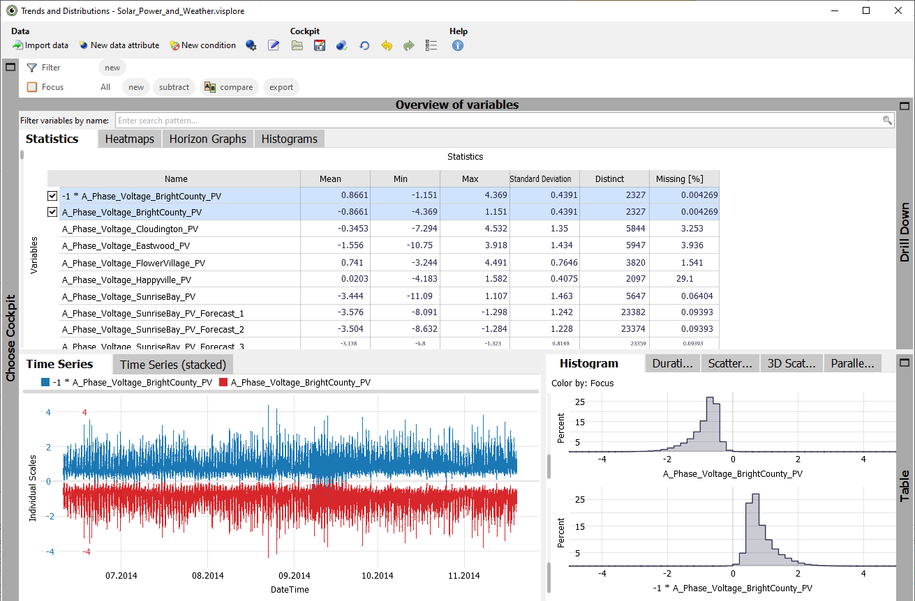
The cockpit updates. You see how the new attribute "-1 * A_Phase_Voltage_BrightCounty_PV" has appeared in the list.
Use the checkmark to select "-1 * A_Phase_Voltage_BrightCounty_PV" in the "Statistics" view. Now, you see the new and the old time series at the same time:
Compute the sum of two inputs
Our next data attribute will be computing the point-wise sum of two time series.
1. Select "A_Phase_Voltage_BrightCounty_PV" and "A_Phase_Voltage_Cloudington_PV" in the "Statistics" view as shown below.
2. Then again, click "New data attribute"
3. Click "Define numeric data attribute".
In the dialog, click in the "Script" field and type: result = i_1 + i_2. Confirm by pressing Compute, and "OK" in the following two dialogs.
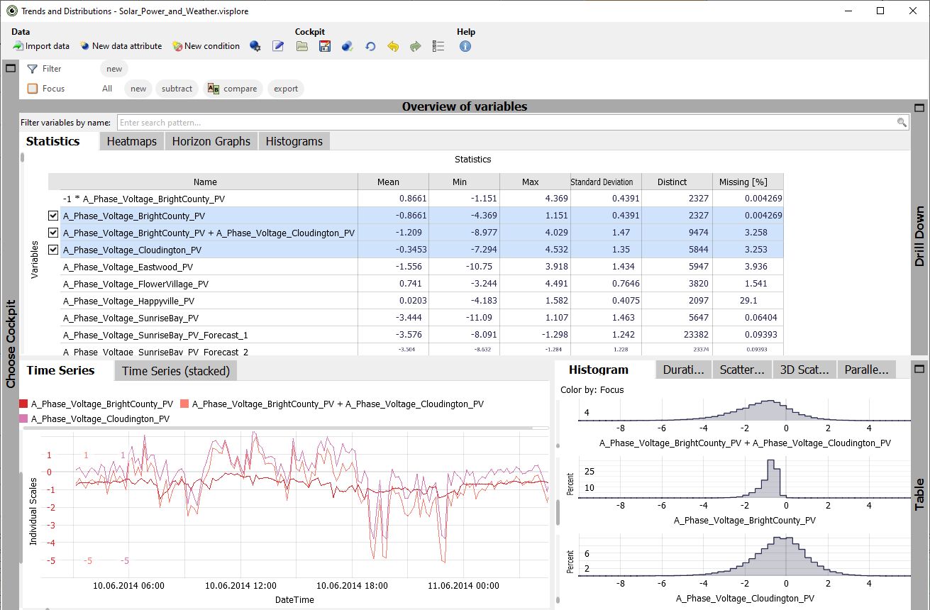
The cockpit updates. When you select the new attribute "A_Phase_Voltage_BrightCounty_PV + A_Phase_Voltage_Cloudington_PV" as third time series, and zoom in a bit (drag right mouse button), Visplore looks like this:
Editing a computation afterwards
You can change the script of a computed data attribute later on. For example, if you discover you made a mistake in the formula, or to tweak some parameters based on what you saw in the visualization.
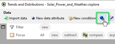
Make sure, the sum attribute "A_Phase_Voltage_BrightCounty_PV + A_Phase_Voltage_Cloudington_PV" is selected in the "Statistics" view, then press the blue icon with the gearwheel in the toolbar:
Now say we want to change the script, as to use the absolute value of the variables before summing them up. For this, we can use one of the built-in formula parts offered at the right side of the dialog:
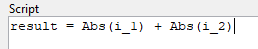
In the "Script" field, delete i_1 from the formula as to look like the image below. Then, hover the word "Abs" in the list of formula parts on the right, and press the right icon with the green arrow, to insert the formula part for taking absolute values.

Do the same to take absolutes of i_2 in the script as well. You may have to adjust the script by hand, as the built-in formula always writes i_1. It should look like this:
Press "Compute" to validate the correctness of the script.
Whenever you edit the script, and press "Compute", the visualizations immediately update with the new values. With this, experimenting with the script and tweaking parameters becomes very efficient.
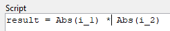
Try out another change: simply replace the + in the formula by typing a * instead, to perform multiplication instead of summation. When pressing "Compute", see how Visplore updates.
Change it back to a '+', as we actually wanted a summation of absolutes, and press "Compute" again.
Important: Now press "Apply" to close the dialog, and thereby confirm the changes you made to the attribute. Pressing "Discard" would discard all changes we made in the dialog, leaving the attribute as before.
Some more examples of scripts
Here is a list of some formulas that may be helpful. Experiment a bit with them, and try to create some of your own. If you want to skip this now, continue to next section.
Examples of simple formulas typed by hand:| Duplicate to use attribute under different name | result = i |
| Difference of two attributes | result = i_1 - i_2 |
| Divison of two attributes | result = i_1 / i_2 |
| Point-wise average of three attributes | result = (i_1 + i_2 + i_3) / 3 |
| Point-wise square | result = i * i |
| Cubic polynomial from one variable | result = (0.3 * i**3) + (0.5 * i**2) + (3 * i) - 7 #remark: i**3 computes i to the power of three. |
Examples of built-in formulas (use the button
 next to a built-in formula for detailed info about parameters):
| Moving average | result = MovingAverage(i, window=10, windowtype="datarecords", symmetric=True, order=i_order) |
| First derivative | result = Derive(i, order=i_order, method="centraldifferences") |
| Time-shift by constant value (here: 2 hours) | result = TimeShift(i, axis=i_order, shift=datetime.timedelta(hours=2)) |
| Time-shift to maximize correlation with other attribute | result = AutoAlign(i_1, basevector=i_2, axis=i_order, maxshiftleft=100, maxshiftright=0) |
| Uniform binning (produces a categorical data attribute) | result = UniformBinning(i, num_bins=10) |
Remember: you can technically type any Python 3 scripts in here, including loops, if-statements and others. Combining Python with built-in formulas is also possible.
Variations: create multiple attributes at once
Now assume we have a number of data attributes, and all of them need to be transformed in the same way before we can do an analysis with them. Say, a number of pressure time series need to be smoothed by a moving average, as the goal is correlating their overall trends and not noise in the data. Creating variations allows you to define the script for one attribute at first, and then applying the same computation to many others at once.
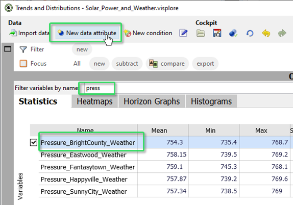
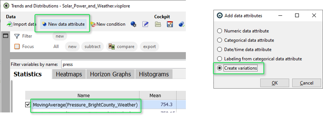
Type "pressure" in the field "Filter variables by name" above the "Statistics" view. Then, select the first time series "Pressure_BrightCounty_Weather", and click "New data attribute" / "Define numeric data attribute":
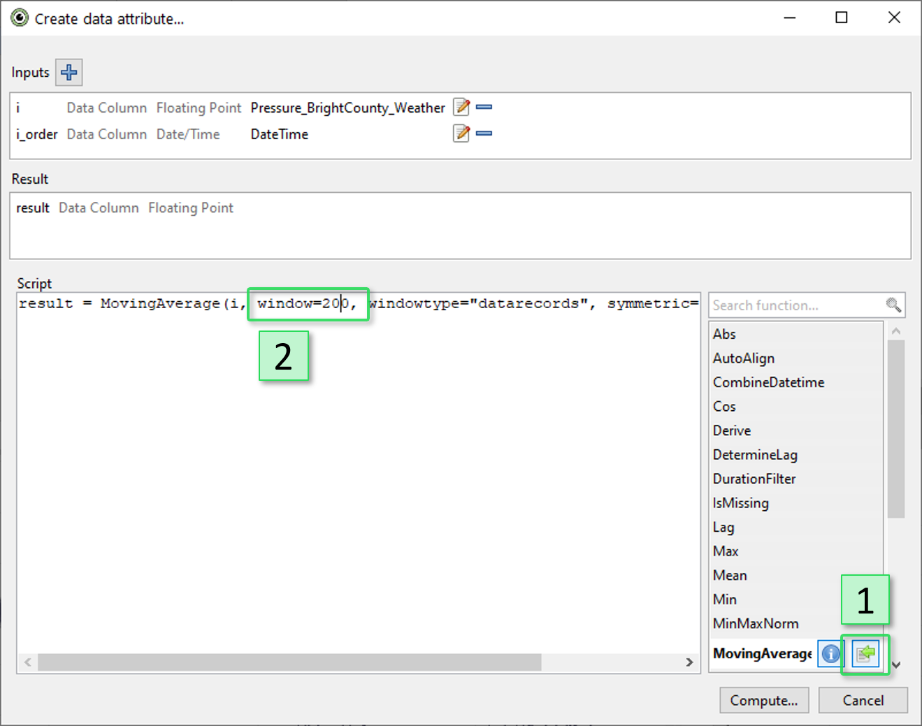
1. In the dialog, press the green icon next to the built-in formula "MovingAverage", to use it in the script (see image below).
2. Before computing, change the parameter "window=10" to "window=200", defining a filter kernel of 200 data records instead of 10, for a much stronger smoothing (see image below).
Confirm by pressing "Compute", then OK in the following dialogs.
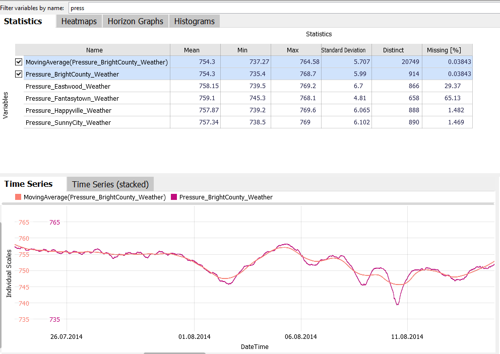
When looking at the original and the smoothed pressure time series together, it looks like this (here, we zoomed a bit).
Now we want to apply the same smoothing to the other pressure time series as well.
Select only the time series "MovingAverage(Pressure_BrightCounty_Weather)" by clicking its name (not the checkbox). Then, click "New data attribute", and choose "Create variations".
This shows a small dialog where you can select the data attributes you want to apply the script to (see image below, left).
Click "Select input for i". Then, search for all variables containing "pressure" in their name, and select all of them except the "Pressure_BrightCounty_Weather", as we computed its smoothed variant already.
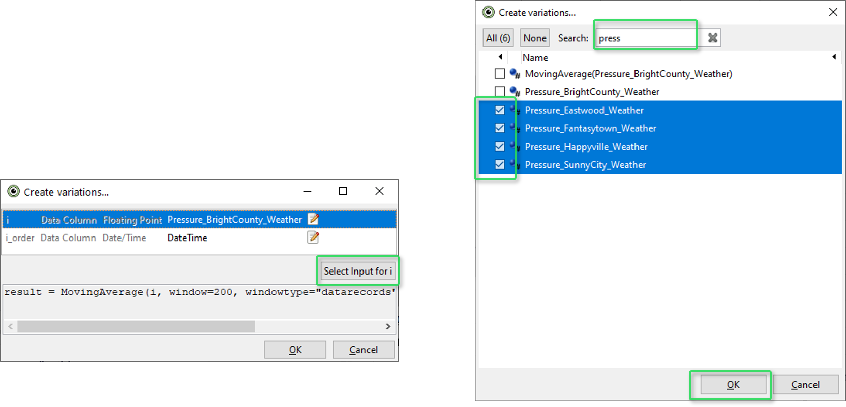
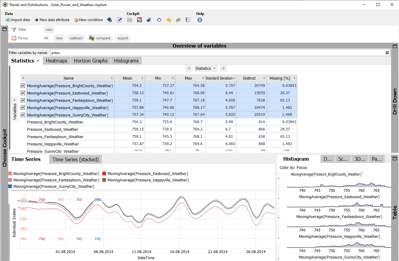
Confirm all dialogs with "OK" until the cockpit updates. Select all time series with "MovingAverage" in their name, such that Visplore looks as follows:
Create a scripted condition
As the final part of the lesson, we experiment with a formula-based way of selecting/labeling subsets of data records. Think of it as scripting a query, like "select all data where time series X is below time series Y", for example. Then, these conditions can be used in the analysis - for example, to see how often the condition occurs, and how it is distributed across categories.
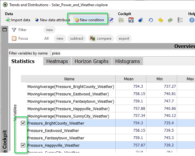
Select the two pressure time series "Pressure_BrightCounty_Weather" and "Pressure_Happyville_Weather". Then, click "New condition" in the toolbar:
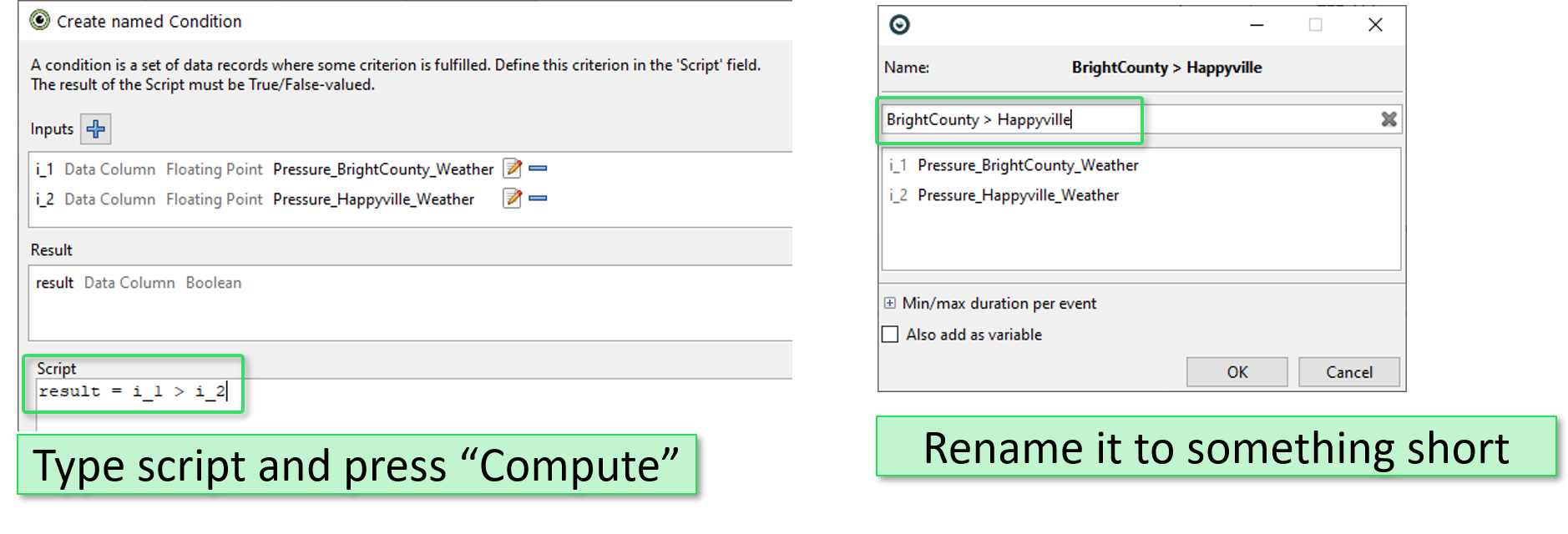
The shown dialog can be used in the same way as the dialog for creating new data attributes. The only difference is that the output here is a boolean (= logical, or binary) array, and not a numerical or categorical one.
In the "Script" field, type: result = i_1 > i_2
Confirm with "Compute"/ "OK". Give it a shorter name, like "BrightCounty > Happyville", and confirm with "OK".
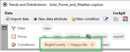
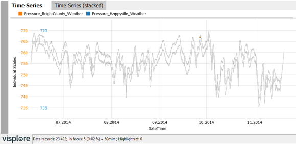
Visplore then shows the condition in the upper area as an orange shape:
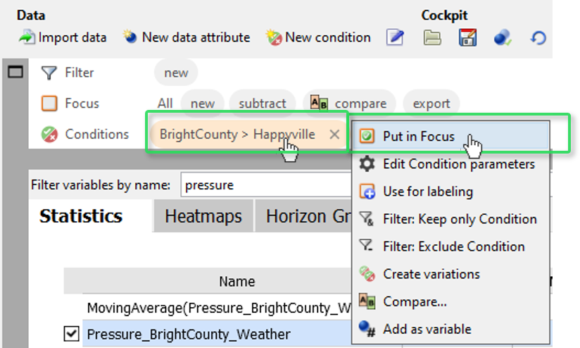
Finally, we want to see how often this condition occurs:
Click the orange shape of the condition we just created, then choose "Put in focus".
Now, the times where the condition is fulfilled are in focus. We see in the footer bar of Visplore, that this only happens at 5 timestamps, corresponding to 50 minutes of the data. The "Time series" view highlights these points.
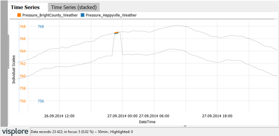
Zoom in to these points in the "Time Series" view by dragging a rectangle around them with the right mouse button, to inspect this rare case in detail (see image above).
It appears, this is a rare condition appearing due to a data artifact rather than in a plausible way.
You can also dynamically edit the script of a condition. Click the orange shape of the condition  , and choose "Edit condition parameters". This allows for dynamically querying your data, and seeing in real-time how often it occurs, how it distributes, etc.
Well done! You have mastered the longest lesson so far - creating new data attributes and new conditions, which takes the flexibility of the analysis to whole new level! :) By the way, when you save your session, all the created data attributes and conditions are kept, so that you can apply the same analysis again when you get new data in two weeks.
>> Continue with Lesson 7: Export images and data
License Statement for the Photovoltaic and Weather dataset used for Screenshots:
"Contains public sector information licensed under the Open Government Licence v3.0."
Source of Dataset (in its original form): https://data.london.gov.uk/dataset/photovoltaic--pv--solar-panel-energy-generation-data
License: UK Open Government Licence OGL 3: http://www.nationalarchives.gov.uk/doc/open-government-licence/version/3/
Dataset was modified (e.g. columns renamed) for easier communication of Visplore USPs.